Neural networks that incorporate BayesForge to quantify uncertainty in their predictions.
General Principles
To model complex, non-linear relationships between variables, we can utilize various approaches, including splines, polynomials, Gaussian processes, and neural networks. Here, we focus on the Bayesian Neural Network (BNN). Think of a neural network as a highly flexible function composed of interconnected layers of neurons 🛈. Each connection possesses a weight, and each neuron has a bias. These weights and biases act as a vast set of adjustable knobs. In a standard neural network, the goal is to find the single best setting for these knobs to map inputs to outputs. Conversely, a BNN learns distributions over its weights and biases rather than single optimal values. This allows the model to capture not only the patterns in the data but also its own uncertainty regarding those patterns.
To construct a BNN, we must define:
A Network Architecture: This specifies the structural design—the number of layers, the number of neurons per layer 🛈, and the activation functions (e.g., ReLU, tanh) that introduce non-linearity. This defines the arrangement of our “knobs.”
Priors for Arrays of Weights and Biases: In simple models like linear regression, we define a prior for each individual parameter (e.g., the slope \beta). However, neural networks often contain thousands or millions of parameters, making it impractical to define a unique prior for each one. Instead, we define priors that act as templates for entire arrays of parameters. For instance, we might specify that all weights in a given layer are drawn from the same Normal(0, 1) distribution. This allows us to efficiently quantify our beliefs about the entire set of network parameters.
An Output Distribution (Likelihood): This defines the probability of the observed data given the network’s predictions. For continuous variables (regression), this is typically a Normal distribution with a variance term \sigma, which quantifies the noise of the data around the model’s predictions.
Considerations
Caution
Uncertainty: Like all Bayesian models, BNNs explicitly account for model parameter uncertainty 🛈. Here, the parameters are the network’s weights (W) and biases (b). We quantify uncertainty through their posterior distribution 🛈. Consequently, we must declare prior distributions 🛈 for all weights and biases, as well as for the output variance \sigma.
Interpretation: Unlike in a linear regression where the coefficient \beta has a direct interpretation (e.g., the change in Y given a unit increase in X), the individual weights and biases in a BNN are not directly interpretable. A single weight’s influence is entangled with thousands of others through non-linear functions. Therefore, BNNs should be viewed as powerful predictive tools rather than explanatory ones. They excel at learning complex topologies and quantifying predictive uncertainty, but if the goal is to isolate the effect of a specific variable, a simpler model is often more appropriate.
Prior distributions: are built following these considerations:
As the data is typically scaled 🛈 (see introduction), we can use a standard Normal distribution (mean 0, standard deviation 1) as a weakly-informative prior for all weights and biases. This acts as a form of regularization.
Since the output variance \sigma must be positive, we can use a positively-defined distribution, such as the Exponential or Half-Normal.
BNNs can be used for both regression and classification. The final layer’s activation and the chosen likelihood distribution depend on the task. For binary classification, a sigmoid activation is paired with a Bernoulli likelihood, which requires a link function 🛈 (logit) to connect the linear output of the network to the probability space [0, 1]. For regression, the identity activation is often used with a Gaussian likelihood.
Computational Scalability: Strictly applying Bayes’ theorem to update the posterior distribution becomes computationally intractable for very large neural networks. Calculating the model evidence (the denominator in Bayes’ rule) requires integrating over a parameter space that may contain millions of dimensions. Furthermore, the posterior landscape in deep networks is often highly non-convex and multimodal. Consequently, sampling algorithms (such as MCMC) may suffer from poor mixing or become “stuck” in local modes, failing to explore the full posterior. In such high-dimensional scenarios, practitioners often must rely on approximate methods, such as Variational Inference 🛈 or Stochastic Gradient MCMC 🛈, to ensure convergence.
Example
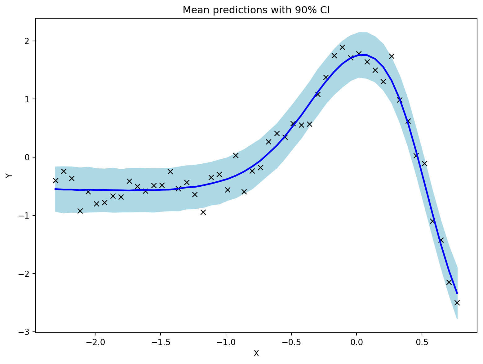
Below is an example code snippet demonstrating a Bayesian Neural Network for regression using the BayesForge (BF) package. Simulated data consist of two continuous variables (Y and X), and the goal is to predict X from Y using a non-linear model.
from BayesForge import bfimport jsonimport jax.numpy as jnpimport matplotlib.pyplot as plt# Setup device------------------------------------------------m = bf(platform='cpu')# Import Data & Data Manipulation ------------------------------------------------withopen('BNN.json', 'r', encoding='utf-8') asfile:# Load the JSON data into a Python dictionary data = json.load(file)# X is already scaledX = jnp.array(data['X']) # Note X shape = (N,2) where first column is the intercept and second column is the predictorY = jnp.array(data['Y']) # Note Y shape = (N,1) where N is the number of observationsm.data_on_model =dict(X = X, Y = Y)# Define model ------------------------------------------------def model(X, Y, D_H=5, D_Y=1): N, D_X = X.shape# First hidden layer: Transforms input to N × D_H (hidden units) w1 = m.bnn.layer_linear( X, dist=m.dist.normal(0, 1, name='w1',shape=(D_X,D_H) ), activation='tanh' )# sample final layer of weights and neural network output# Final layer (z3) computes linear combination of second hidden layer w2 = m.bnn.layer_linear( X=w1, dist=m.dist.normal(0, 1, name='w2',shape=(D_H,D_Y)) ) sigma = m.dist.exponential(1, name='sigma') m.dist.normal(w2, sigma, obs=Y,name='Y')# Run mcmc ------------------------------------------------m.fit(model, progress_bar=False) # Approximate posterior distributions for weights, biases, and sigma# Predictions from the model ------------------------------------------------pred = m.sample(samples =500)['Y']pred = pred[..., 0]mean_prediction = jnp.mean(pred, axis=0)percentiles = jnp.percentile(pred, jnp.array([5.0, 95.0]), axis=0)# make plotsfig, ax = plt.subplots(figsize=(8, 6), constrained_layout=True)# plot training dataax.plot(X[:, 1], Y[:, 0], "kx")# plot 90% confidence level of predictionsax.fill_between( X[:, 1], percentiles[0, :], percentiles[1, :], color="lightblue")# plot mean predictionax.plot(X[:, 1], mean_prediction, "blue", ls="solid", lw=2.0)ax.set(xlabel="X", ylabel="Y", title="Mean predictions with 90% CI")
/home/sosa/work/3.12venv/lib/python3.10/site-packages/tqdm/auto.py:21: TqdmWarning:

IProgress not found. Please update jupyter and ipywidgets. See https://ipywidgets.readthedocs.io/en/stable/user_install.html
bf v 0.0.48 package loaded
jax.local_device_count 32
⚠️This function is still in development. Use it with caution. ⚠️
⚠️This function is still in development. Use it with caution. ⚠️
⚠️This function is still in development. Use it with caution. ⚠️
⚠️This function is still in development. Use it with caution. ⚠️
⚠️This function is still in development. Use it with caution. ⚠️
⚠️This function is still in development. Use it with caution. ⚠️
/home/sosa/work/BF/BayesForge/Main/main.py:674: UserWarning:

Sample's batch dimension size 4000 is different from the provided 500 num_samples argument. Defaulting to 4000.
⚠️This function is still in development. Use it with caution. ⚠️
⚠️This function is still in development. Use it with caution. ⚠️
library(BayesForge)m=importBF(platform='cpu')# Load csv file# Import data ------------------------------------------------path =normalizePath(paste(system.file(package ="BayesForge"),"/data/BNN.json", sep =''))data <-fromJSON(path)m$data_on_model =list()m$data_on_model$X = jnp$array(data$X)m$data_on_model$Y = jnp$array(data$Y)# Define model ------------------------------------------------model <-function(X, Y, D_X =2, D_H=5L, D_Y=1L){ w1 <- m$bnn$layer_linear(X, dist=bf.dist.normal(0, 1, name='w1',shape=c(D_X,D_H)), activation='tanh') w2 <- m$bnn$layer_linear( w1, dist=bf.dist.normal(0, 1, name='w2',shape=c(D_H,D_Y)),activation='tanh' )# Prior for the output standard deviation s =bf.dist.exponential(1, name ='s')# Likelihoodbf.dist.normal(w2, s, obs = Y)}# Run mcmc ------------------------------------------------m$fit(model) # Approximate posterior distributions
Mathematical Details
In the Bayesian formulation, we place priors 🛈 on all weights and biases and define a likelihood for the output. For a regression task with a K-hidden-layer BNN with J neurons per hidden layer and a D_X-vector of predictors and a D_Y-vector of outcomes we can run the model as below. For simplicity we consider a single hidden layer (as in the code example) with a hyperbolic tangent (\tanh) activation function 🛈, mapped to a linear output layer. Because the input matrix X incorporates the intercept as its first column, the bias term is implicitly included in the layer’s weights:
Y_i is the observed outcome for the i-th observation.
\mu_i is the predicted mean output of the neural network for the i-th observation.
\sigma is the observation noise standard deviation.
X_i is the input row vector for the i-th observation, containing the intercept and the predictor variable. It has length D_X = 2.
H_i is the hidden layer representation vector for the i-th observation. It has length D_H = 5.
W_1 is the weight matrix of the first hidden layer, with a shape of D_X \times D_H (i.e., 2 \times 5).
W_2 is the final layer weight matrix used to compute the linear combination of the hidden layer, with a shape of D_H \times D_Y (i.e., 5 \times 1).
All elements within the weight matrices W_1 and W_2 are assigned independent standard Normal priors.
Notes
Note
The primary difference between a Frequentist and Bayesian neural network lies in how parameters are treated. In the frequentist approach, weights and biases are point estimates found by minimizing a loss function (e.g., via gradient descent). Techniques like Dropout 🛈or L2 regularization 🛈 are often used to prevent overfitting 🛈, which can be interpreted as approximations to a Bayesian treatment. In contrast, the Bayesian formulation does not seek a single best set of weights. Instead, it uses methods like MCMC or Variational Inference to approximate the entire posterior distribution for every weight and bias. This provides a principled and direct way to quantify model uncertainty.
While present an example of non-linear regression, the Bayesian Neural Network can be used for linear regressions as well (keeping in mind that interpretation of the weights are impossible).
Phan, Du, Neeraj Pradhan, and Martin Jankowiak. 2019. “Composable Effects for Flexible and Accelerated Probabilistic Programming in NumPyro.”arXiv Preprint arXiv:1912.11554.